Simple Linear Regression with Python
Contents
Introduction and Data
This brief tutorial shows an example of how to perform linear regression with python. There are many ways to perform linear regression with python. This example uses the SciPy and Pandas libraries that are commonly used in python-based analysis.
The data used in this demonstration is in a CSV file called kfm.csv. The variables are:
| Variable | Description |
|---|---|
no |
A numeric vector, identification number |
dl.milk |
A numeric vector, breast-milk intake (dl/24h) |
sex |
A factor with levels boy and girl |
weight |
A numeric vector, weight of child (kg) |
ml.suppl |
A numeric vector, supplementary milk substitute (ml/24h) |
mat.weight |
A numeric vector, weight of mother (kg) |
mat.height |
A numeric vector, height of mother (cm) |
Data as CSV: Here is the complete data set, in CSV format.
   "no",    "dl.milk",    "sex",    "weight", "ml.suppl", "mat.weight",  "mat.height"
    1,       8.42,    "boy",     5.002,      250,         65,         173
    4,       8.44,    "boy",     5.128,        0,         48,         158
    5,       8.41,    "boy",     5.445,       40,         62,         160
   10,       9.65,    "boy",     5.106,       60,         55,         162
   12,       6.44,    "boy",     5.196,      240,         58,         170
   16,       6.29,    "boy",     5.526,        0,         56,         153
   22,       9.79,    "boy",     5.928,       30,         78,         175
   28,       8.43,    "boy",     5.263,        0,         57,         170
   31,       8.05,    "boy",     6.578,      230,         57,         168
   32,       6.48,    "boy",     5.588,      555,         58,         173
   36,       7.64,    "boy",     4.613,        0,         58,         171
   39,       8.73,    "boy",     5.882,       60,         54,         163
   54,       7.71,    "boy",     5.618,      315,         68,         179
   55,       8.39,    "boy",     6.032,      370,         56,         175
   72,       9.32,    "boy",     6.030,      130,         62,         168
   78,       6.78,    "boy",     4.727,        0,         59,         172
   79,       9.63,    "boy",     5.345,       55,         68,         172
   80,       5.97,    "boy",     5.359,       10,         60,         159
   81,       8.39,    "boy",     5.320,       20,         59,         174
   82,      10.43,    "boy",     6.501,      105,         76,         185
   83,       5.62,    "boy",     4.666,       80,         52,         159
   84,       6.84,    "boy",     4.969,       80,         54,         165
   90,      10.35,    "boy",     6.105,        0,         78,         174
   91,       4.91,    "boy",     4.360,        0,         49,         162
   98,       7.70,    "boy",     5.667,        0,         63,         165
    6,      10.03,   "girl",     6.100,        0,         58,         167
   14,       7.42,   "girl",     5.421,       45,         67,         175
   25,       5.00,   "girl",     4.744,       30,         73,         164
   26,       8.67,   "girl",     5.800,       30,         80,         175
   27,       6.90,   "girl",     5.822,        0,         59,         174
   34,       6.89,   "girl",     5.081,       20,         53,         162
   37,       7.22,   "girl",     5.336,      590,         58,         160
   38,       7.01,   "girl",     5.637,      100,         63,         170
   40,       8.06,   "girl",     5.546,       70,         61,         170
   41,       4.44,   "girl",     4.386,      150,         58,         167
   43,       8.57,   "girl",     5.568,       30,         70,         172
   46,       5.17,   "girl",     5.169,        0,         65,         160
   47,       7.74,   "girl",     4.825,      210,         58,         176
   56,       7.93,   "girl",     5.156,       20,         74,         165
   57,       5.03,   "girl",     4.120,      100,         55,         162
   63,       7.68,   "girl",     4.725,      100,         50,         160
   65,       6.91,   "girl",     5.636,       30,         49,         161
   66,       8.23,   "girl",     5.377,      110,         55,         167
   68,       7.36,   "girl",     5.195,       80,         59,         171
   74,       6.46,   "girl",     5.385,       70,         51,         165
   85,       7.24,   "girl",     4.635,       15,         48,         167
   88,       9.03,   "girl",     5.730,      100,         62,         172
  100,       4.63,   "girl",     5.360,      145,         48,         157
  104,       6.97,   "girl",     4.890,       30,         67,         165
  105,       5.82,   "girl",     4.339,       95,         47,         163
The Task: perform a linear regression using dl.milk as explanatory and weight as response.
Getting Started
iPython Notebook is a very useful python environment for storing notes and performing analysis with embedded images and commentary. The examples in this tutorial were created in iPython Notebook.
To begin, load the libraries needed to perform the analysis.
Installing Libraries: You may need to use easy_install or pip to install these packages. Alternatively, the Anaconda distribution of python includes many of the necessary libraries.
# Import the numpy library
import numpy

# Import the plotting library and refer to it as plt
import matplotlib.pyplot as plt

# Required only for iPython Notebook
%pylab inline

import pandas as pd

# Useful library for working with linear regression
# http://statsmodels.sourceforge.net/stable/generated/statsmodels.regression.linear_model.RegressionResults.html
import statsmodels.formula.api as sm

from scipy import stats

# Use pandas to load the data into a 2D numpy array
data = pd.read_csv("C:/Users/clay/Desktop/py/tutorials/kfm.csv")
# Slice the numpy array to get the data vectors
# 1 represents the second column of data and
# 3 represents the fourth column of data

dlmilk = data.ix[:,1]
weight = data.ix[:,3]
Explore the data: plotting
One of the first steps in exploratory data analysis always is to plot the data. Let’s look at how to plot the data with matplotlib in python. The code is commented. See the Additional References section at the bottom of this post for links to more resources about plotting data in python.
# Weight of the child is the dependent variable here, so we will plot
# it on the y-axis

fig = plt.figure(figsize=(12, 8), dpi=80)
fig.suptitle('dL of Milk vs. Weight of Child', fontsize=16)
theplot  = fig.add_subplot(1,1,1)
theplot.scatter(dlmilk,weight)
theplot.set_xlabel('dL of Milk')
theplot.set_ylabel('Weight of Child')
plt.show()
And here is the resulting plot…
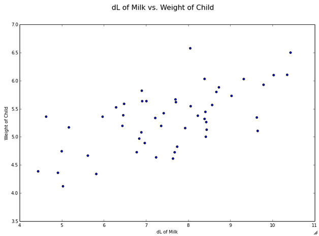
Hey, those look pretty correlated… let’s check it out.
Explore the data: Correlation
There are two ways that we can calculate the correlation between the variables. The first is using the scipy stats library
# Calculates a Pearson correlation coefficient and
# the p-value for testing non-correlation.
stats.pearsonr(dlmilk,weight)
The output:
(0.63604482482603641, 6.9153761747038878e-07)
According to the SciPy reference guide, the stats.pearsonr(x,y) function “Calculates a Pearson correlation coefficient and the p-value for testing non-correlation.” Note that this is a 2-tailed p-value.
So, in our results above, our correlation coefficient is 0.636, indicating strong correlation between temps and chirps. The p-value for the test of non-correlation is very small, so we reject the null hypothesis that the values are not correlated and conclude that they are correlated.
We can also use Panda, but it does not provide a p-value for the test:
# Pandas approach -- no p-value
weight.corr(dlmilk)

# There are optional parameters for kendall tau and spearman
# weight.corr(dlmilk, method='spearman') for example
The output:
0.63604482482603653
Building a Linear Model
Pandas points us to the statsmodels package for detailed linear regression output:
# Approach to OLS with more results
# http://pandas.pydata.org/pandas-docs/dev/remote_data.html
import statsmodels.formula.api as smf
model  = smf.ols("weight ~ dlmilk", data)
fitted = model.fit()
print fitted.summary()
The results:
                            OLS Regression Results
==============================================================================
Dep. Variable:                 weight   R-squared:                       0.405
Model:                            OLS   Adj. R-squared:                  0.392
Method:                 Least Squares   F-statistic:                     32.61
Date:                Fri, 13 Dec 2013   Prob (F-statistic):           6.92e-07
Time:                        12:44:57   Log-Likelihood:                -27.434
No. Observations:                  50   AIC:                             58.87
Df Residuals:                      48   BIC:                             62.69
Df Model:                           1
==============================================================================
                 coef    std err          t      P>|t|      [95.0% Conf. Int.]
------------------------------------------------------------------------------
Intercept      3.5873      0.309     11.603      0.000         2.966     4.209
dlmilk         0.2307      0.040      5.711      0.000         0.149     0.312
==============================================================================
Omnibus:                        0.477   Durbin-Watson:                   1.948
Prob(Omnibus):                  0.788   Jarque-Bera (JB):                0.628
Skew:                           0.164   Prob(JB):                        0.731
Kurtosis:                       2.560   Cond. No.                         39.8
==============================================================================
Alternatively, we can use the features built into Pandas for different output:
# OLS with pandas
# Build the model and fit it
model = pd.ols(y = weight, x = dlmilk)
model
The results:
-------------------------Summary of Regression Analysis-------------------------

Formula: Y ~ <x> + <intercept>

Number of Observations:         50
Number of Degrees of Freedom:   2

R-squared:         0.4046
Adj R-squared:     0.3921

Rmse:              0.4275

F-stat (1, 48):    32.6117, p-value:     0.0000

Degrees of Freedom: model 1, resid 48

-----------------------Summary of Estimated Coefficients------------------------
      Variable       Coef    Std Err     t-stat    p-value    CI 2.5%   CI 97.5%
--------------------------------------------------------------------------------
             x     0.2307     0.0404       5.71     0.0000     0.1515     0.3099
     intercept     3.5873     0.3092      11.60     0.0000     2.9813     4.1932
---------------------------------End of Summary---------------------------------
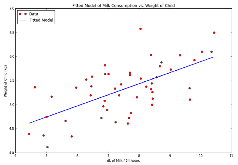
Building off of the first approach, let’s plot the data again, this time with the fitted line:
# Plot the data again, with the fitted line
plt.figure(figsize=(12, 8), dpi=80)
plt.plot(dlmilk,weight, 'ro')
plt.plot(dlmilk,fitted.fittedvalues, 'b')

# For a Lowess smoothed line
# http://statsmodels.sourceforge.net/devel/generated/statsmodels.nonparametric.smoothers_lowess.lowess.html

# loc = 2 puts the legend in the upper-left
# http://matplotlib.org/users/legend_guide.html
plt.legend(['Data', 'Fitted Model'], loc = 2)

# Set axis limits
# plt.ylim(12,22)
# plt.xlim(65,98)

plt.xlabel('dL of Milk / 24 hours')
plt.ylabel('Weight of Child (kg)')
plt.title('Fitted Model of Milk Consumption vs. Weight of Child')
plt.show()
Verifying Assumptions
When performing linear regression, we have several assumptions to check:
1. Linearity: There is a linear relationship between the independent and dependent variables. (The mean of the Y values is accurately modeled by a linear function of the X values)
2. Normality of the Errors: The random error term is assumed to have a normal distribution with a mean of zero.
3. Homoscedasticity: The random error term is assumed to have a constant variance.
4. Independence of the Errors: The errors are independent of each other.
5. No Perfect Multicollinearity: (For multiple linear regression) There is no perfect collinearity between independent variables.
Let’s look at these one-by-one.
Linearity of the Relationship
Well, this one is easy and we’ve already done it. Simply examine the plot that we previously created and you can see linearity in the relationship, versus a curve that might indicate a quadratic relationship.
Normality of the Residuals
We can formally test the residuals for normality using a Shapiro Wilk test:
# Formal test -- Shapiro Wilk
stats.shapiro(fitted.norm_resid())
The results:
(0.9769636392593384, 0.43218812346458435)
The null hypothesis is that the residuals are normal. The second value returned in the results is the p-value, which indicates that we fail to reject our null and conclude that the residuals are normal.
(Insert a Q-Q plot here later…)
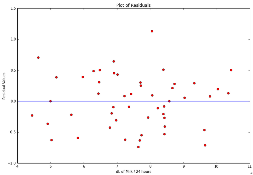
Homoscedasticity
Here’s how we check the homoscedasticity of the residuals:
# Check residuals
# http://statsmodels.sourceforge.net/devel/examples/generated/example_gls.html

residuals = fitted.resid

plt.figure(figsize=(12, 8), dpi=80)
plt.plot(dlmilk,residuals, 'ro')

# Add a horizontal line at 0
# http://matplotlib.org/api/pyplot_api.html#matplotlib.pyplot.axhline
plt.axhline(y=0, xmin=0, xmax=1)

plt.xlabel('dL of Milk / 24 hours')
plt.ylabel('Residual Values')
plt.title('Plot of Residuals')

plt.show()
We do not see any type of fan shape in the residuals, which indicates that the residuals exhibit homoscedasticity.
Independence of the Error Terms
We want a Durbin-Watson test result that is close to 2. If you look at the regression output above, you will see that the value for our model is 1.948.
To test it separately, do the following:
import statsmodels as ssm
ssm.stats.stattools.durbin_watson(fitted.resid)
The result:
1.9476337892720015
No Perfect Multicollinearity
We only have one independent variable, so we do not need to test for perfect multicollinearity.
Additional Tests: Influential Points
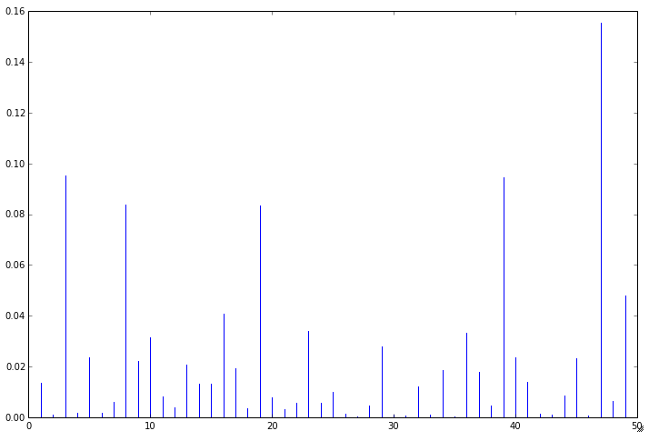
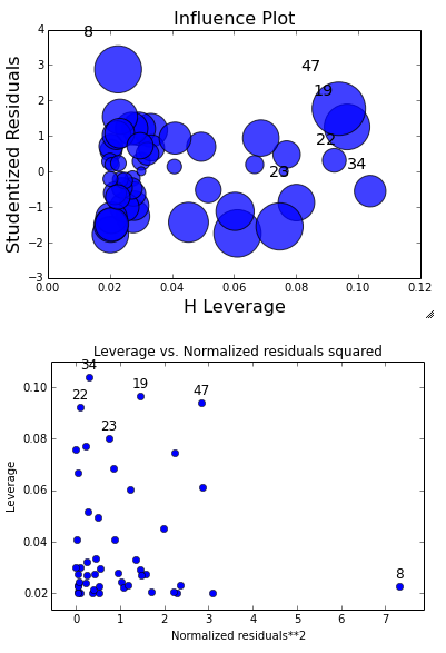
There are several additional tests that we can perform and plots that we can generate to help identify influential points in the data:
influence = fitted.get_influence()

# c is the distance and p is p-value
(c,p) = influence.cooks_distance

plt.figure(figsize=(12, 8), dpi=80
plt.stem(np.arange(len(c)), c, markerfmt=",")
plt.show()
# Looking at leverage - need to import this package
from statsmodels.graphics.regressionplots import *

plot_leverage_resid2(fitted)
influence_plot(fitted)
Additional References
Plotting with Matplotlib
