Decision Trees with R

Introduction and Data

This example demonstrates how to perform decision tree analysis using R. The dataset used in this demonstration is titled beetles. The variables are:

Data as CSV: Here is the complete data set, in CSV format.

The Task: Using only the provided measurements of a beetle’s aedeagus, determine the species of beetle from the genus Chaetocnoma. The three species are concinna (Con), heikertingeri (Hei), and heptapotamica (Hep).

Getting Started in R

To begin, you need to have R installed on your computer. You can download it at the R Project website. We also recommend the R Studio. Launch R and then type the following commands at the command line.

#You may need to install the following packages

install.packages("party")

#Load the package into R.  This can also
#be done by clicking "Packages" and selecting
#the data set

library(party)

#Read the csv into R

beetles=read.csv("beetles.csv", header=TRUE)

Partitioning the Data

Since the goal of this procedure is to predict a categorical variable based on numeric inputs, a decision tree may be appropriate here.

First, the data must be separated into training and validation sets. A common percentage for these datasets is 70% training and 30% validation. The training dataset will be used to build the decision tree, while the validation set will be used to test the predictions and evaluate the model.

set.seed(1234)
train<-sample(2,nrow(beetles),replace=TRUE,prob=c(0.7,0.3))
beetles.tr<-beetles[train==1,]
beetles.va<-beetles[train==2,]

Building the Decision Tree

Now that the data are separated, the decision tree may be created. The commands below create a decision tree with the default settings.

model<-Species~Width+Angle
beetles_tree<-ctree(model,data=beetles.tr)
table(predict(beetles_tree),beetles.tr$Species)

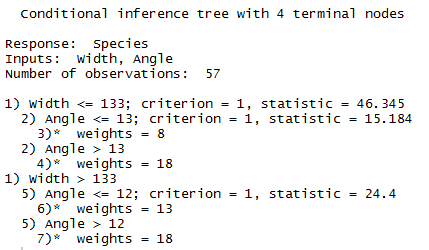
The output shows that the tree possesses clear predictive power, as the species are almost completely predicted correctly. Printing the tree reveals the decision rules and properties.

print(beetles_tree)

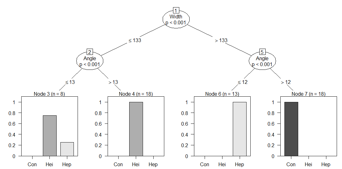
The first split was on aedeagus width of 133 microns. Both of these divisions were then split again on Angle (one at 12, and the other at 13). The weights output reveals how many observations are present in a particular leaf. To get more detailed information, the tree may be plotted.

plot(beetles_tree)

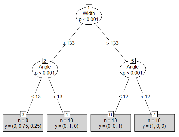
All of the information is still available from the print function, but additional insights are provided. The p-values are available at each split, as well as bar graphs of the species divisions within leaves. Notice that it is not possible to get exact percentages of species within leaves. For example, Node 3 contains approximately 75% heikertingeri. For a similar chart with percentages, the type can be specified as “simple”.

plot(beetles_tree, type="simple")

This chart reveals that the proportion of heikertingeri in Node 3 is, in fact, 75%.

Validation of the Model

Now, the model must be tested against the validation data. This allows one to see how the model responds to new data, and serves as an assessment of the model’s validity if implemented.

beetles_treetest<-predict(beetles_tree, newdata=beetles.va)
table(beetles_treetest, beetles.va$Species)

The model seems to perform well on the validation set, correctly predicting all but one specimen.

Conclusion

We hope you found this guide to decision trees in R useful!