Simple Linear Regression with R
Contents
Introduction and Data
This example demonstrates how to perform simple linear regression using R. The data used in this demonstration is housed in the ISwR package and is titled kfm. The variables are:
| Variable | Description |
|---|---|
no |
A numeric vector, identification number |
dl.milk |
A numeric vector, breast-milk intake (dl/24h) |
sex |
A factor with levels boy and girl |
weight |
A numeric vector, weight of child (kg) |
ml.suppl |
A numeric vector, supplementary milk substitute (ml/24h) |
mat.weight |
A numeric vector, weight of mother (kg) |
mat.height |
A numeric vector, height of mother (cm) |
Data as CSV: Here is the complete data set, in CSV format.
   "no",    "dl.milk",    "sex",    "weight", "ml.suppl", "mat.weight",  "mat.height"
    1,       8.42,    "boy",     5.002,      250,         65,         173
    4,       8.44,    "boy",     5.128,        0,         48,         158
    5,       8.41,    "boy",     5.445,       40,         62,         160
   10,       9.65,    "boy",     5.106,       60,         55,         162
   12,       6.44,    "boy",     5.196,      240,         58,         170
   16,       6.29,    "boy",     5.526,        0,         56,         153
   22,       9.79,    "boy",     5.928,       30,         78,         175
   28,       8.43,    "boy",     5.263,        0,         57,         170
   31,       8.05,    "boy",     6.578,      230,         57,         168
   32,       6.48,    "boy",     5.588,      555,         58,         173
   36,       7.64,    "boy",     4.613,        0,         58,         171
   39,       8.73,    "boy",     5.882,       60,         54,         163
   54,       7.71,    "boy",     5.618,      315,         68,         179
   55,       8.39,    "boy",     6.032,      370,         56,         175
   72,       9.32,    "boy",     6.030,      130,         62,         168
   78,       6.78,    "boy",     4.727,        0,         59,         172
   79,       9.63,    "boy",     5.345,       55,         68,         172
   80,       5.97,    "boy",     5.359,       10,         60,         159
   81,       8.39,    "boy",     5.320,       20,         59,         174
   82,      10.43,    "boy",     6.501,      105,         76,         185
   83,       5.62,    "boy",     4.666,       80,         52,         159
   84,       6.84,    "boy",     4.969,       80,         54,         165
   90,      10.35,    "boy",     6.105,        0,         78,         174
   91,       4.91,    "boy",     4.360,        0,         49,         162
   98,       7.70,    "boy",     5.667,        0,         63,         165
    6,      10.03,   "girl",     6.100,        0,         58,         167
   14,       7.42,   "girl",     5.421,       45,         67,         175
   25,       5.00,   "girl",     4.744,       30,         73,         164
   26,       8.67,   "girl",     5.800,       30,         80,         175
   27,       6.90,   "girl",     5.822,        0,         59,         174
   34,       6.89,   "girl",     5.081,       20,         53,         162
   37,       7.22,   "girl",     5.336,      590,         58,         160
   38,       7.01,   "girl",     5.637,      100,         63,         170
   40,       8.06,   "girl",     5.546,       70,         61,         170
   41,       4.44,   "girl",     4.386,      150,         58,         167
   43,       8.57,   "girl",     5.568,       30,         70,         172
   46,       5.17,   "girl",     5.169,        0,         65,         160
   47,       7.74,   "girl",     4.825,      210,         58,         176
   56,       7.93,   "girl",     5.156,       20,         74,         165
   57,       5.03,   "girl",     4.120,      100,         55,         162
   63,       7.68,   "girl",     4.725,      100,         50,         160
   65,       6.91,   "girl",     5.636,       30,         49,         161
   66,       8.23,   "girl",     5.377,      110,         55,         167
   68,       7.36,   "girl",     5.195,       80,         59,         171
   74,       6.46,   "girl",     5.385,       70,         51,         165
   85,       7.24,   "girl",     4.635,       15,         48,         167
   88,       9.03,   "girl",     5.730,      100,         62,         172
  100,       4.63,   "girl",     5.360,      145,         48,         157
  104,       6.97,   "girl",     4.890,       30,         67,         165
  105,       5.82,   "girl",     4.339,       95,         47,         163
The Task: perform a linear regression using dl.milk as explanatory and weight as response.
Getting Started in R
To begin, you need to have R installed on your computer. You can download it at the R Project website. We also recommend the R Studio. Launch R and then type the following commands at the command line.
#You may need to install the following packages

# Data sets and scripts for text examples and exercises in P. Dalgaard (2008), 'Introductory Statistics with R', 2nd ed., Springer Verlag, ISBN 978-0387790534.
install.packages("ISwR")

# This package accompanies J. Fox and S. Weisberg, An R Companion to Applied Regression, Second Edition, Sage, 2011.
install.packages("car")

# MASS-Functions and datasets to support Venables and Ripley, 'Modern Applied Statistics with S' (4th edition, 2002).
install.packages("MASS")

#Load the ISwR package into R.  This can also
#be done by clicking "Packages" and selecting
#the data set

library(ISwR)
library(car)
library(MASS)

#Attach the data set

attach(kfm)
Explore the data: Plotting
One of the most important first steps in any data analysis is to plot the data. The following code can be used to create a scatterplot in R.
Note: When using multiple lines of R, it may be best to write a script rather than the command prompt.
#Create a Scatterplot of the data

plot(dl.milk,weight,main="Linear Regression of Weight on Breastfeeding",
xlab="Breast Milk Intake (dl/day)",
ylab="Weight (kg)",
pch=19)

#Add the regression line and a lowess

model<-lm(weight~dl.milk)
abline(model,col="red")
lines(lowess(dl.milk,weight),col="blue")
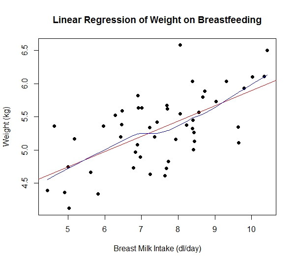
The scatterplot does show evidence of a positive linear trend, indicating that as the amount of daily breast milk intake increases, weight tends to increase. The red line is the least squares regression line, which will be discussed in greater detail in just a moment. The blue line is the lowess (locally weighted scatterplot smoothing) line, which also tries to fit a line to the scatterplot. If this line is not relatively straight, it may indicate that simple linear regression (without any sort of transformation of variables) is not appropriate. In this case, the lowess appears relatively straight. In fact, it appears to be very close to the least square regression line. All of this indicates that simple linear regression may be appropriate.
Explore the data: Correlation
Correlation is a measure of the strength and direction of a linear relationship. The farther from 0 (and closer to 1 or -1), the stronger the relationship. The sign indicates whether the relationship is positive or negative.
#find correlation
cor(dl.milk,weight)
The correlation is determined to be .636, indicating a moderately strong, positive, linear relationship. This supports the conclusions made above.
Verifying Assumptions
When performing linear regression, we have several assumptions to check:
1. Linearity: There is a linear relationship between the independent and dependent variables. (The mean of the Y values is accurately modeled by a linear function of the X values)
2. Normality of the Errors: The random error term is assumed to have a normal distribution with a mean of zero.
3. Homoscedasticity: The random error term is assumed to have a constant variance.
4. Independence of the Errors: The errors are independent of each other.
5. No Perfect Multicollinearity: (For multiple linear regression) There is no perfect collinearity between independent variables.
Let’s look at these one-by-one.
Linearity of the Relationship
It is necessary to assume that the mean of the response is a linear combination of the predictor variables. This can be demonstrated visually through the use of a component and residual plot.
#Evaluating Nonlinearity
crPlots(model)
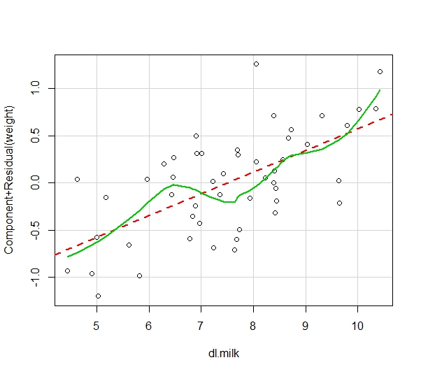
The Component+Residual Plot highlights the linearity of the mean. Therefore, this condition is met.
Normality of the Residuals
It is important to assume that the residuals of the regression line are normally distributed. Though this assumption can often be rejected using a visual approach (in the case of residuals that are clearly non-normal), it is more appropriate to use a formal test for normality. The code below plots a Q-Q Plot and histogram, as well as performing a Shapiro-Wilk test for Normality.
#Evaluating assumption of Normality of Residuals

qqPlot(model, main="QQ Plot")
dev.new()
sresid <- studres(model)
hist(sresid, freq=FALSE, main="Distribution of Studentized Residuals")
xfit<-seq(min(sresid),max(sresid),length=40)
yfit<-dnorm(xfit)
lines(xfit, yfit)
shapiro.test(sresid)
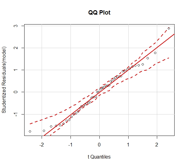
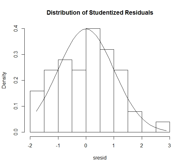
There is no reason to doubt the Normality of the residuals, as the Q-Q Plot appears linear and the histogram is relatively Normal. Furthermore, the Shapiro-Wilk Test for Normality (Null Hypothesis is that data are from a Normally distributed population) provides a w-statistic of .9775. This corresponds to a p-value of .4533, which is not sufficient to reject the hypothesis of Normality. Therefore, it is concluded that the residuals are Normally distributed.
Homoscedasticity
It is also important to verify that the variance of errors is relatively constant across all levels of the independent variable. The Breusch-Pagan Test of Non-Constant Error Variance is one way of verifying this assumption. If the condition is not met, a Spread-Level Plot can be used to determine an appropriate transformation.
#Evaluating assumption of Homoskedasticity
ncvTest(model)
spreadLevelPlot(model)
Here are the results:
Non-constant Variance Score Test
Variance formula: ~ fitted.values
Chisquare = 0.1806033    Df = 1     p = 0.6708552
The Breusch-Pagan Test provides a very small chi-square statistic (.1806 at df=1). This corresponds to a p-value of .67, which is not significant to reject the null hypothesis of constant variance. The Spread-Level Plot suggests a cubic transformation of the independent variable, though this result is meaningless due to the results of the Breusch-Pagan Test.
Independence of the Error Terms
A Durbin-Watson test is one way to assess the condition of whether or not the errors are independent of each other. The null hypothesis is that the errors are independent (ie. They are not correlated).
#Evaluating Independence
durbinWatsonTest(model)
The results:
 lag Autocorrelation D-W Statistic p-value
   1    -0.009624478      1.947634     0.9
 Alternative hypothesis: rho != 0
The Durbin-Watson test yields a statistic of about 1.95, which corresponds to a p-value of .876. This is not enough to reject the null hypothesis, so it is concluded that the errors are, indeed, independent.
No Perfect Multicollinearity
It is important to assume that there is no perfect collinearity between independent variables. This condition does not apply to this particular example, since there is only one predictor variable. The code below illustrates how to calculate the Variance Inflation Factors in the event where this would be relevant. Keep in mind that if the square root of any variance inflation factor is greater than two, this condition may be violated.
Note: This code will produce an error with this model because there is only one predictor variable.
#Evaluating Multicollinearity (For models of two or more terms)
vif(model)
sqrt(vif(model)) > 2 # problem?
Performing Simple Linear Regression
Now that all of the preliminary work has been completed, regression analysis can begin. There are a few things that can be completed to this end. The linear regression can provide an equation for the least squares regression line, which can then be used to interpolate or extrapolate predictions for weight. A confidence interval can be calculated for the intercept and the independent variables. Also, an ANOVA table can be constructed. The code below competes all of these tasks.
#perform simple linear regression

summary(model)
confint(model,level=.95)
anova(model)
The results:
> summary(model)

Call:
lm(formula = weight ~ dl.milk)

Residuals:
     Min       1Q   Median       3Q      Max
-0.73703 -0.29640  0.03133  0.30044  1.13338

Coefficients:
            Estimate Std. Error t value Pr(>|t|)
(Intercept)   3.5873     0.3092  11.603 1.56e-15 ***
dl.milk       0.2307     0.0404   5.711 6.92e-07 ***
---
Signif. codes:  0 '***' 0.001 '**' 0.01 '*' 0.05 '.' 0.1 ' ' 1

Residual standard error: 0.4275 on 48 degrees of freedom
Multiple R-squared:  0.4046,  Adjusted R-squared:  0.3921
F-statistic: 32.61 on 1 and 48 DF,  p-value: 6.915e-07
The output from the summary function begins with a reminder of the regression model. This is followed by the five-number summary of the residuals. Next, R displays a table indicating the coefficients and relative significance. Here it can be seen that the coefficient of the dl.milk variable is .2307 and it is significant, since the p-value is much less than .05 (6.9E-7). The least-squares regression line is only explaining about 40% of the variation, as indicated by the R-squared value.
> confint(model,level=.95)
                2.5 %    97.5 %
(Intercept) 2.9656584 4.2088989
dl.milk     0.1494911 0.3119612
The 95% confidence intervals indicate that the true intercept is estimated to be between 2.97 and 4.21, while the true coefficient of dl.milk is between 0.15 and 0.31.
> anova(model)
Analysis of Variance Table

Response: weight
          Df Sum Sq Mean Sq F value    Pr(>F)
dl.milk    1 5.9595  5.9595  32.612 6.915e-07 ***
Residuals 48 8.7716  0.1827
---
Signif. codes:  0 '***' 0.001 '**' 0.01 '*' 0.05 '.' 0.1 ' ' 1
So the equation of the least squares regression line is
weight = 3.5873 + dl.milk*0.2307
This can be used to create a data set of predictions as follows:
predmilk<-seq(0,10,by=.2)
predweight<-(3.5873+predmilk*.2307)
pred<-cbind(predmilk,predweight)
head(pred)
The console shows the first 5 of the predictions:
     predmilk predweight
[1,]      0.0    3.58730
[2,]      0.2    3.63344
[3,]      0.4    3.67958
[4,]      0.6    3.72572
[5,]      0.8    3.77186
[6,]      1.0    3.81800
Further Exploration—Influential Points and Outliers
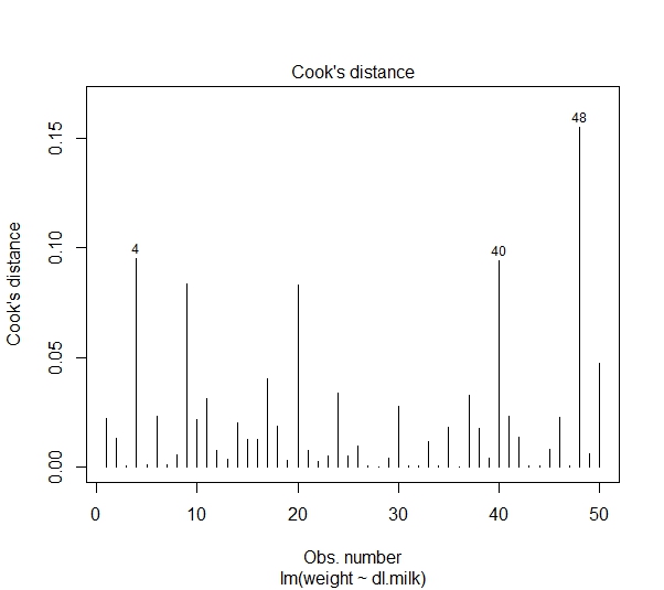
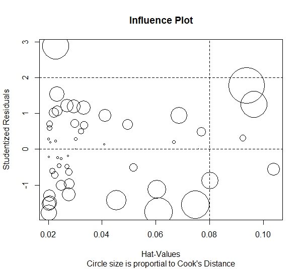
The following code uses Cook’s D and an influential plot to determine which points may be influential or outliers.
#Influential Points
avPlots(model)
cutoff <- 4/(nrow(mtcars)-length(model$coefficients)-2)
plot(model, which=4, cook.levels=cutoff)
influencePlot(model, id.method="noteworthy", main="Influence Plot", sub="Circle size is proportial to Cook's Distance")
The Cook’s D plot reveals that observations 4, 40, and 48 are influential observations.
Conclusion
We hope you found this guide to simple linear regression in R useful!
